Prais–Winsten estimation
In econometrics, Prais–Winsten estimation is a procedure meant to take care of the serial correlation of type AR(1) in a linear model. It is a modification of Cochrane–Orcutt estimation in the sense that it does not lose the first observation and leads to more efficiency as a result.
Contents |
Theory
Consider the model
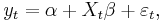
where  is the time series of interest at time t,
  is a vector of coefficients,
  is a matrix of explanatory variables, and
  is the error term. The error term can be serially correlated over time:
 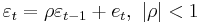 and
and  is a white noise. In addition to the Cochrane–Orcutt procedure transformation, which is

for t=2,3,...,T, Prais-Winsten procedure makes a reasonable transformation for t=1 in the following form

Then the usual least squares estimation is done.
Estimation procedure
To do the estimation in a compact way it is directive to look at the auto-covariance function of the error term considered in the model above:
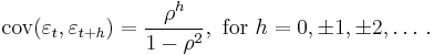
Now is easy to see that the variance-covariance,  , of the model is
![\mathbf{\Omega} = \begin{bmatrix}
\frac{1}{1-\rho^2} & \frac{\rho}{1-\rho^2} & \frac{\rho^2}{1-\rho^2} & \cdots & \frac{\rho^{T-1}}{1-\rho^2} \\[8pt]
\frac{\rho}{1-\rho^2} & \frac{1}{1-\rho^2} & \frac{\rho}{1-\rho^2} & \cdots & \frac{\rho^{T-2}}{1-\rho^2} \\[8pt]
\frac{\rho^2}{1-\rho^2} & \frac{\rho}{1-\rho^2} & \frac{1}{1-\rho^2} & \cdots & \frac{\rho^{T-2}}{1-\rho^2} \\[8pt]
\vdots & \vdots & \vdots & \ddots & \vdots \\[8pt]
\frac{\rho^{T-1}}{1-\rho^2} & \frac{\rho^{T-2}}{1-\rho^2} & \frac{\rho^{T-3}}{1-\rho^2} & \cdots & \frac{1}{1-\rho^2}
\end{bmatrix}.](/2012-wikipedia_en_all_nopic_01_2012/I/2469f2f978721869f1e8c51525b8cbb9.png)
Now having  (or an estimate of it), we see that,
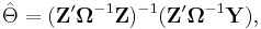
where  is a matrix of observations on the independent variable (Xt, t = 1, 2, ..., T) including a vector of ones,
  is a vector stacking the observations on the dependent variable (Xt, t = 1, 2, ..., T) and
  includes the model parameters.
Note
To see why the initial observation assumption stated by Prais-Winsten (1954) is reasonable, considering the mechanics of general least square estimation procedure sketched above is helpful. The inverse of can be decomposed as 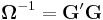 with
with
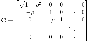
A pre-multiplication of model in a matrix notation with this matrix gives the transformed model of Prais-Winsten.
Restrictions
The error term is still restricted to be of an AR(1) type. If is not known, a recursive procedure maybe used to make the estimation feasible. See Cochrane–Orcutt estimation.
References
- Prais, S. J.; Winsten, C. B. (1954), Trend Estimators and Serial Correlation [1]
- Wooldridge, J. (2008) Introductory Econometrics: A Modern Approach, 4th Edition, South-Western Pub. ISBN 0324660545 (p. 435)